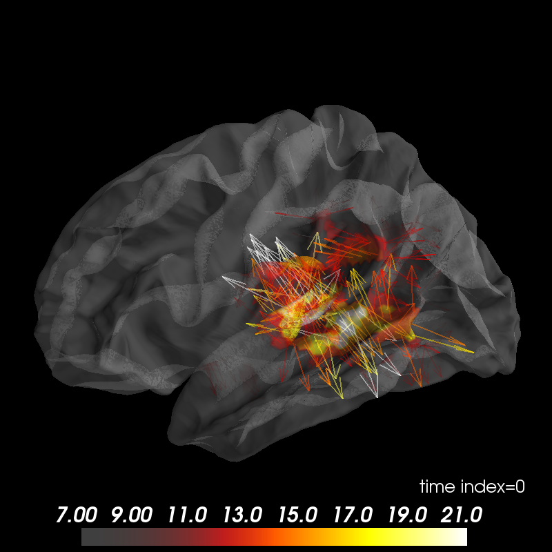
Plot vector-valued MEG inverse solution

Data were computed using mne-python (http://martinos.org/mne).

import os
import numpy as np

from surfer import Brain, TimeViewer  # noqa, analysis:ignore
from surfer.io import read_stc

print(__doc__)

# Do some basic things: define subject, surface and hemisphere(s) to plot,
# and create the :class:`surfer.viz.Brain` object.

subject_id, surf = 'fsaverage', 'white'
hemi = 'lh'
brain = Brain(subject_id, hemi, surf, size=(800, 800), interaction='terrain',
              cortex='0.5', alpha=0.5, show_toolbar=True, units='m')

# Read the MNE dSPM inverse solution

hemi = 'lh'
stc_fname = os.path.join('example_data', 'meg_source_estimate-' +
                         hemi + '.stc')
stc = read_stc(stc_fname)

# data and vertices for which the data is defined
data = stc['data']
vertices = stc['vertices']
time = np.linspace(stc['tmin'], stc['tmin'] + data.shape[1] * stc['tstep'],
                   data.shape[1], endpoint=False)

# MNE will soon add the option for a "full" inverse to be computed and stored.
# In the meantime, we can get the equivalent for our data based on the
# surface normals:

data_full = brain.geo['lh'].nn[vertices][..., np.newaxis] * data[:, np.newaxis]

# Now we add the data and set the initial time displayed to 100 ms:
brain.add_data(data_full, colormap='hot', vertices=vertices, alpha=0.5,
               smoothing_steps=5, time=time, hemi=hemi, initial_time=0.1,
               vector_alpha=0.5, verbose=False)

# scale colormap
brain.scale_data_colormap(fmin=7, fmid=14, fmax=21, transparent=True,
                          verbose=False)

# viewer = TimeViewer(brain)