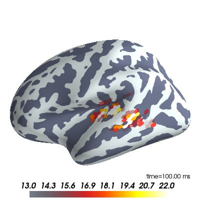
Plot MEG inverse solution

Data were computed using mne-python (http://martinos.org/mne)

import os
import numpy as np

from surfer import Brain
from surfer.io import read_stc

print(__doc__)

Set up some useful variables and make the plot.

# define subject, surface and hemisphere(s) to plot:

subject_id, surf = 'fsaverage', 'inflated'
hemi = 'lh'

# create Brain object for visualization
brain = Brain(subject_id, hemi, surf, size=(400, 400), background='w',
              interaction='terrain', cortex='bone', units='m')

# label for time annotation in milliseconds


def time_label(t):
    return 'time=%0.2f ms' % (t * 1e3)


# Read MNE dSPM inverse solution and plot

for hemi in ['lh']:  # , 'rh']:
    stc_fname = os.path.join('example_data', 'meg_source_estimate-' +
                             hemi + '.stc')
    stc = read_stc(stc_fname)

    # data and vertices for which the data is defined
    data = stc['data']
    vertices = stc['vertices']

    # time points (in seconds)
    time = np.linspace(stc['tmin'], stc['tmin'] + data.shape[1] * stc['tstep'],
                       data.shape[1], endpoint=False)

    # colormap to use
    colormap = 'hot'

    # add data and set the initial time displayed to 100 ms,
    # plotted using the nearest relevant colors
    brain.add_data(data, colormap=colormap, vertices=vertices,
                   smoothing_steps='nearest', time=time, time_label=time_label,
                   hemi=hemi, initial_time=0.1, verbose=False)

# scale colormap
brain.scale_data_colormap(fmin=13, fmid=18, fmax=22, transparent=True,
                          verbose=False)

To change the time displayed to 80 ms uncomment this line:

# brain.set_time(0.08)

uncomment these lines to use the interactive TimeViewer GUI

# from surfer import TimeViewer
# viewer = TimeViewer(brain)